Saul Dobilas 2022-02-21
对门控循环单元(Gated Recurrent Units)的可视化解释,并附带一个使用真实数据的端到端 Python 示例。
神经网络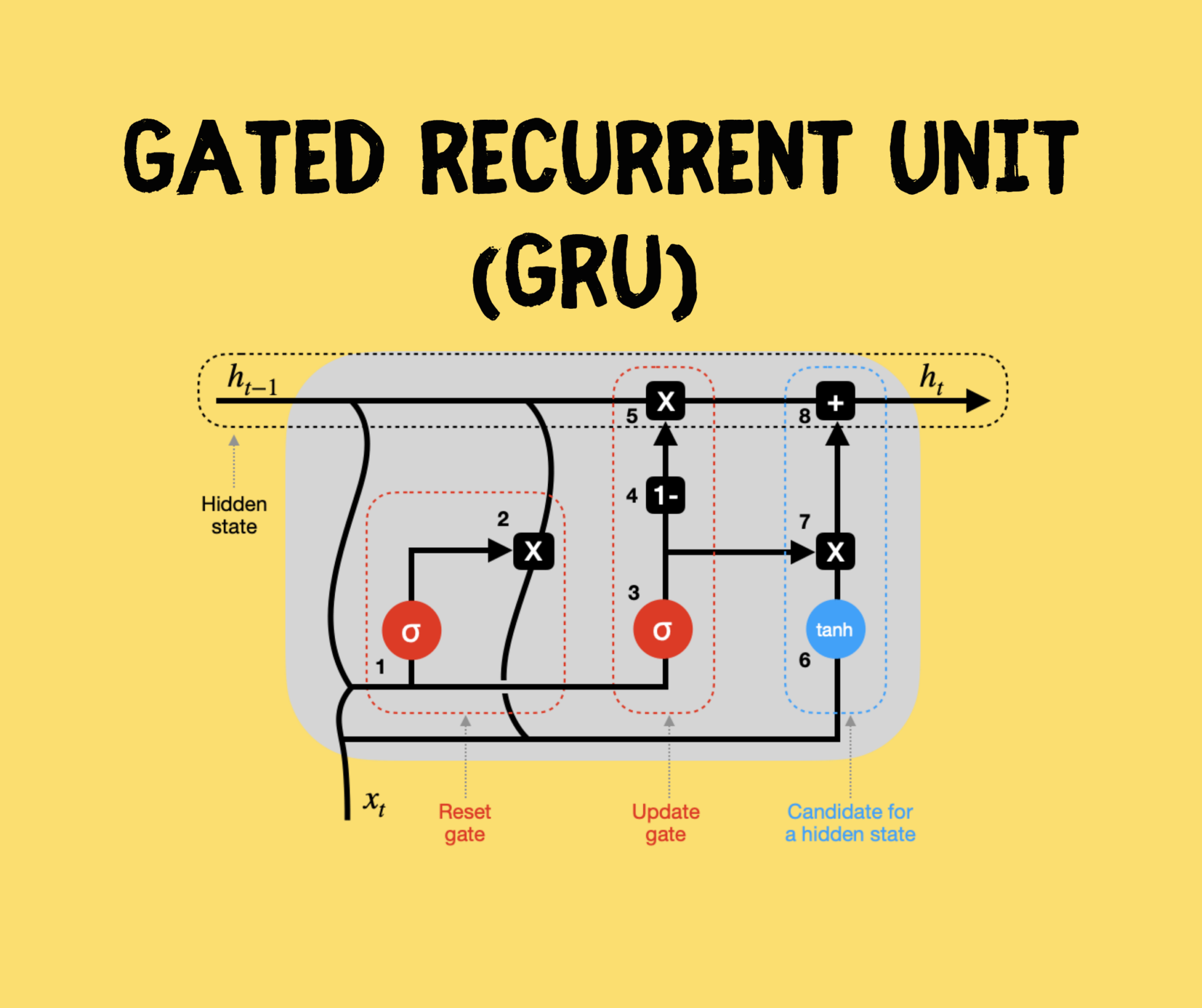 门控循环单元(GRU)。来源
引言
门控循环单元(GRU)和长短期记忆网络(LSTM)被提出,旨在解决标准循环神经网络(RNN)中存在的梯度消失/爆炸问题。
在本文中,我将为你概述 GRU 的架构,并提供一个详细的 Python 示例,你可以用它来构建自己的 GRU 模型。
目录
- GRU 在机器学习宇宙中的位置
- GRU 是如何构建的?它与标准 RNN 和 LSTM 有何不同?
- 使用 Keras 和 TensorFlow 库构建 GRU 神经网络的完整 Python 示例
GRU 在机器学习宇宙中的位置
下图是我尝试对最常见机器学习算法进行分类的结果。
虽然我们经常以监督方式使用神经网络(即使用带标签的训练数据),但我认为神经网络独特的机器学习方法值得单独归为一类。
因此,在我的图表中,神经网络(NNs)从机器学习宇宙的核心分支出来。循环神经网络(RNNs)是 NNs 的一个子分支,包含标准 RNN、LSTM 和 GRU 等算法。
GRU 是如何构建的?它与标准 RNN 和 LSTM 有何不同?
让我们先回顾一下典型的 RNN 结构:它包含输入层、隐藏层和输出层。注意,你可以拥有任意数量的节点,下面的 2–3–2 设计仅用于说明。
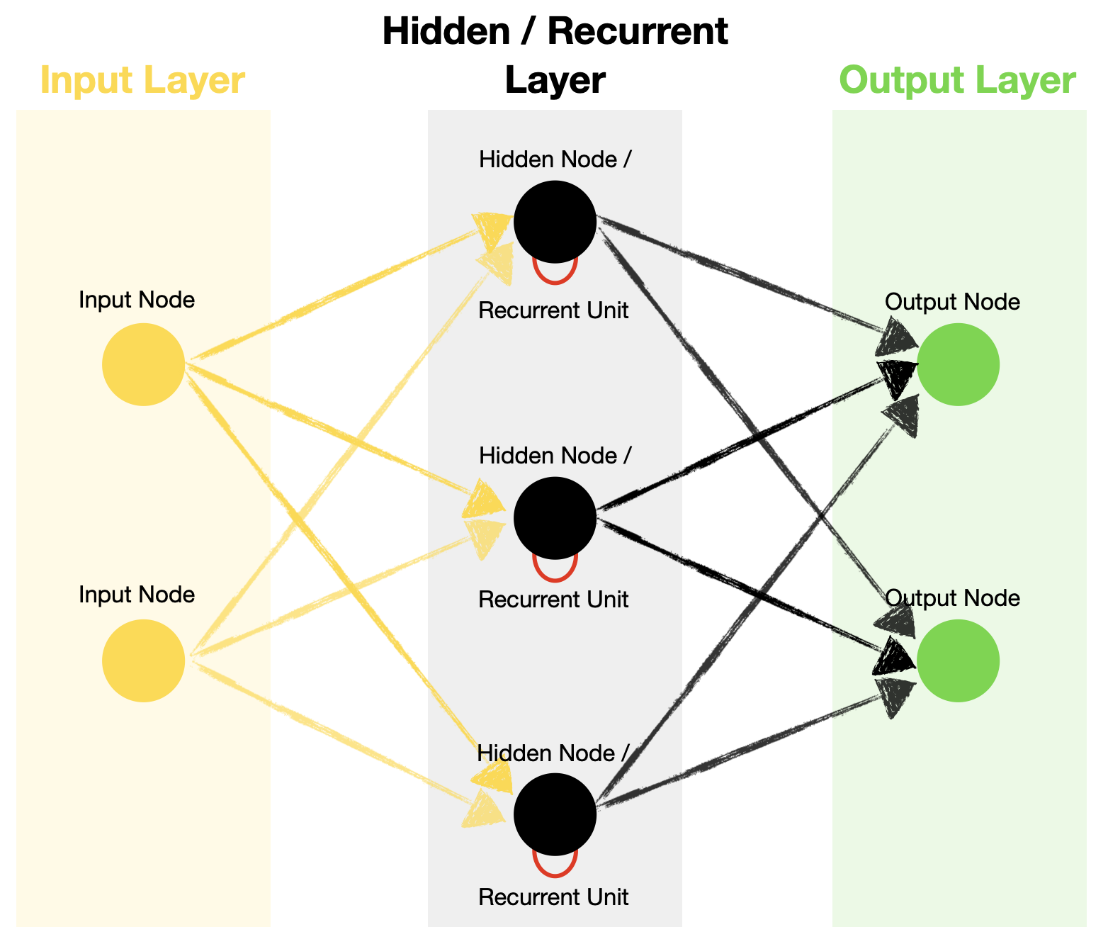 标准循环神经网络架构。来源
与前馈神经网络不同,RNN 在其隐藏层中包含循环单元,这使得算法能够处理序列数据。这是通过将前一时间步的隐藏状态递归地传递,并与当前时间步的输入相结合来实现的。
时间步(Timestep) – 对输入通过循环单元的一次处理。时间步的数量等于序列的长度。
标准 RNN 与 LSTM 中的循环单元架构
我们知道,RNN 利用循环单元从序列数据中学习,这对三种类型(标准 RNN、LSTM 和 GRU)都成立。
然而,它们在循环单元内部的运作方式却大不相同。
例如,标准 RNN 使用隐藏状态来记住信息。而 LSTM 和 GRU 引入了“门”机制,用于控制哪些信息应被记住、哪些应被遗忘,然后再更新隐藏状态。此外,LSTM 还有一个细胞状态(cell state),作为长期记忆。
以下是标准 RNN 和 LSTM 的简化循环单元图(未显示权重和偏置)。看看它们之间的对比。
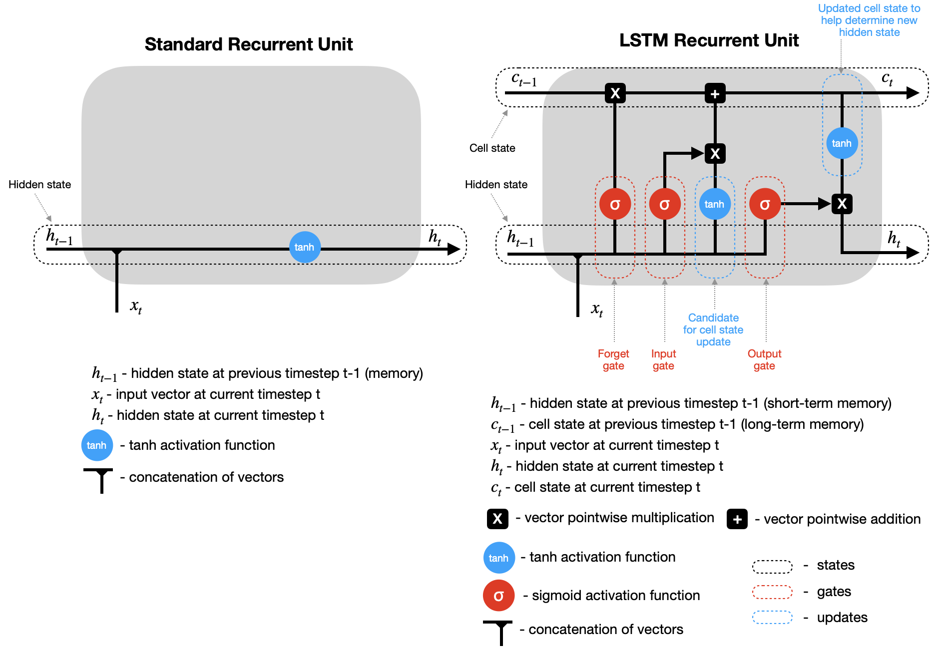 标准循环单元 vs. LSTM 循环单元。来源
请注意,在这两种情况下,在时间步 t 计算出隐藏状态(以及 LSTM 的细胞状态)后,它们会被传回循环单元,并与时间步 t+1 的输入结合,以计算时间步 t+1 的新隐藏状态(和细胞状态)。此过程会重复进行,直到达到预设的时间步数 n(即 t+2, t+3, …, t+n)。
GRU 是如何工作的?
GRU 与 LSTM 类似,但门更少。此外,它仅依赖隐藏状态在循环单元之间传递记忆,因此没有单独的细胞状态。让我们详细分析这个简化的 GRU 图(未显示权重和偏置)。
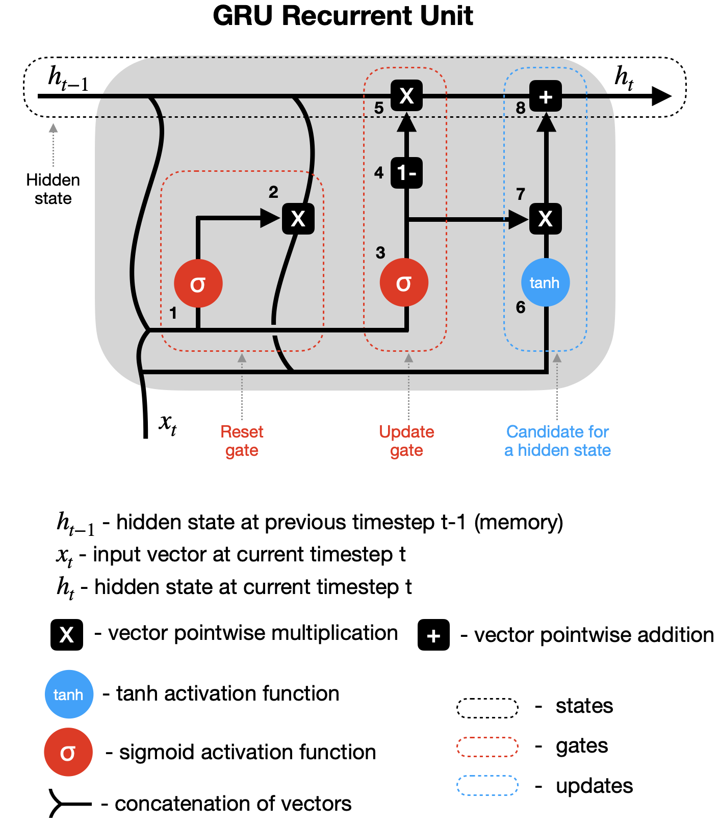 GRU 循环单元。来源
1–2 重置门(Reset gate) – 前一隐藏状态(h_{t-1})和当前输入(x_t)被组合(分别乘以其权重并加上偏置),然后通过重置门。由于 sigmoid 函数的取值范围在 0 到 1 之间,第一步决定了哪些值应被丢弃(0)、记住(1)或部分保留(介于 0 和 1 之间)。第二步将前一隐藏状态与第一步的输出相乘,从而重置它。
3–4–5 更新门(Update gate) – 第三步看似与第一步类似,但请注意,用于缩放这些向量的权重和偏置是不同的,因此会产生不同的 sigmoid 输出。因此,在将组合向量通过 sigmoid 函数后,我们将其从全 1 向量中减去(第四步),再与前一隐藏状态相乘(第五步)。这是用新信息更新隐藏状态的一部分。
6–7–8 候选隐藏状态(Hidden state candidate) – 在第二步重置前一隐藏状态后,其输出与新输入(x_t)结合,乘以其各自的权重并加上偏置,然后通过 tanh 激活函数(第六步)。接着,候选隐藏状态与更新门的结果相乘(第七步),并与之前修改过的 h_{t-1} 相加,形成新的隐藏状态 h_t。
接下来,该过程在时间步 t+1 等处重复,直到循环单元处理完整个序列。
使用 Keras 和 TensorFlow 库构建 GRU 神经网络的 Python 示例
现在,我们将使用 GRU 创建一个多对多(many-to-many)预测模型,即使用一个序列的值来预测下一个序列。注意,GRU 也可用于一对一(不推荐,因为这不是序列数据)、多对一(many-to-one)和一对多(one-to-many)的设置。
数据准备
首先,我们需要获取以下数据和库:
- 来自 Kaggle 的澳大利亚天气数据(许可证:Creative Commons,原始数据来源:澳大利亚联邦气象局)
- Pandas 和 Numpy 用于数据处理
- Plotly 用于数据可视化
- TensorFlow/Keras 用于 GRU 神经网络
- Scikit-learn 库用于数据缩放(MinMaxScaler)
让我们导入所有库:
# Tensorflow / Keras
from tensorflow import keras # for building Neural Networks
print('Tensorflow/Keras: %s' % keras.__version__) # print version
from keras.models import Sequential # for creating a linear stack of layers for our Neural Network
from keras import Input # for instantiating a keras tensor
from keras.layers import Bidirectional, GRU, RepeatVector, Dense, TimeDistributed # for creating layers inside the Neural Network

# Data manipulation
import pandas as pd # for data manipulation
print('pandas: %s' % pd.__version__) # print version
import numpy as np # for data manipulation
print('numpy: %s' % np.__version__) # print version

# Sklearn
import sklearn
print('sklearn: %s' % sklearn.__version__) # print version
from sklearn.preprocessing import MinMaxScaler # for feature scaling

# Visualization
import plotly
import plotly.express as px
import plotly.graph_objects as go
print('plotly: %s' % plotly.__version__) # print version
上述代码打印了我在本示例中使用的包版本:
Tensorflow/Keras: 2.7.0
pandas: 1.3.4
numpy: 1.21.4
sklearn: 1.0.1
plotly: 5.4.0
接下来,下载并加载澳大利亚天气数据(来源:Kaggle)。我们只加载所需的部分列,因为整个数据集对我们的模型来说并不必要。
同时,我们进行一些简单的数据处理,并派生出两个新变量:年-月(Year-Month)和中位温度(Median Temperature)。
# Set Pandas options to display more columns
pd.options.display.max_columns=150

# Read in the weather data csv - keep only the columns we need
df=pd.read_csv('weatherAUS.csv', encoding='utf-8', usecols=['Date', 'Location', 'MinTemp', 'MaxTemp'])

# Drop records where target MinTemp=NaN or MaxTemp=NaN
df=df[pd.isnull(df['MinTemp'])==False]
df=df[pd.isnull(df['MaxTemp'])==False]

# Convert dates to year-months
df['Year-Month']= (pd.to_datetime(df['Date'], yearfirst=True)).dt.strftime('%Y-%m')

# Derive median daily temperature (mid point between Daily Max and Daily Min)
df['MedTemp']=df[['MinTemp', 'MaxTemp']].median(axis=1)

# Show a snaphsot of data
df
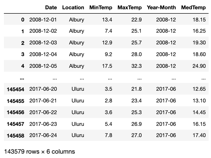 Kaggle 澳大利亚天气数据片段(含部分修改)。来源
目前,我们每个地点和日期都有一条中位温度记录。然而,日温度波动很大,使得预测更加困难。因此,我们计算每月平均值,并将数据转置,使地点作为行、年-月作为列。
# Create a copy of an original dataframe
df2=df[['Location', 'Year-Month', 'MedTemp']].copy()

# Calculate monthly average temperature for each location
df2=df2.groupby(['Location', 'Year-Month'], as_index=False).mean()

# Transpose dataframe
df2_pivot=df2.pivot(index=['Location'], columns='Year-Month')['MedTemp']

# Remove locations with lots of missing (NaN) data
df2_pivot=df2_pivot.drop(['Dartmoor', 'Katherine', 'Melbourne', 'Nhil', 'Uluru'], axis=0)

# Remove months with lots of missing (NaN) data
df2_pivot=df2_pivot.drop(['2007-11', '2007-12', '2008-01', '2008-02', '2008-03', '2008-04', '2008-05', '2008-06', '2008-07', '2008-08', '2008-09', '2008-10', '2008-11', '2008-12', '2017-01', '2017-02', '2017-03', '2017-04', '2017-05', '2017-06'], axis=1)

# Display the new dataframe
df2_pivot
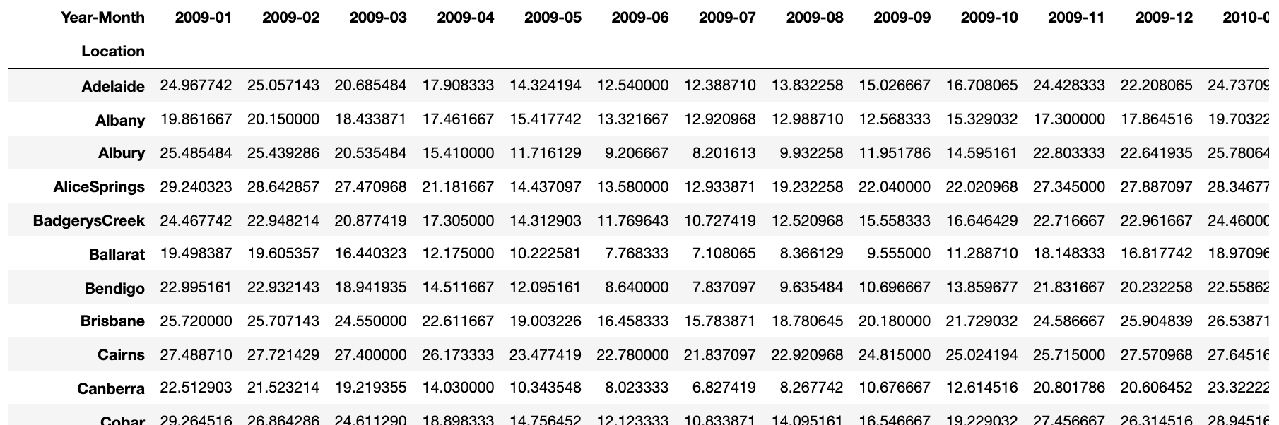 按地点和月份划分的平均月温度。来源
由于我们使用的是真实数据,注意到有三个月份(2011–04、2012–12 和 2013–02)在数据框中完全缺失。因此,我们通过取前后月份的平均值来填补这些缺失月份。
# Add missing months 2011-04, 2012-12, 2013-02 and impute data
df2_pivot['2011-04']=(df2_pivot['2011-03']+df2_pivot['2011-05'])/2
df2_pivot['2012-12']=(df2_pivot['2012-11']+df2_pivot['2013-01'])/2
df2_pivot['2013-02']=(df2_pivot['2013-01']+df2_pivot['2013-03'])/2

# Sort columns so Year-Months are in the correct order
df2_pivot=df2_pivot.reindex(sorted(df2_pivot.columns), axis=1)
最后,我们可以将数据绘制成图表。
# Plot average monthly temperature derived from daily medians for each location
fig = go.Figure()
for location in df2_pivot.index:
    fig.add_trace(go.Scatter(x=df2_pivot.loc[location, :].index,
                             y=df2_pivot.loc[location, :].values,
                             mode='lines',
                             name=location,
                             opacity=0.8,
                             line=dict(width=1)
                            ))

# Change chart background color
fig.update_layout(dict(plot_bgcolor = 'white'), showlegend=True)

# Update axes lines
fig.update_xaxes(showgrid=True, gridwidth=1, gridcolor='lightgrey',
                 zeroline=True, zerolinewidth=1, zerolinecolor='lightgrey',
                 showline=True, linewidth=1, linecolor='black',
                 title='Date'
                )

fig.update_yaxes(showgrid=True, gridwidth=1, gridcolor='lightgrey',
                 zeroline=True, zerolinewidth=1, zerolinecolor='lightgrey',
                 showline=True, linewidth=1, linecolor='black',
                 title='Degrees Celsius'
                )

# Set figure title
fig.update_layout(title=dict(text="Average Monthly Temperatures", font=dict(color='black')))

fig.show()
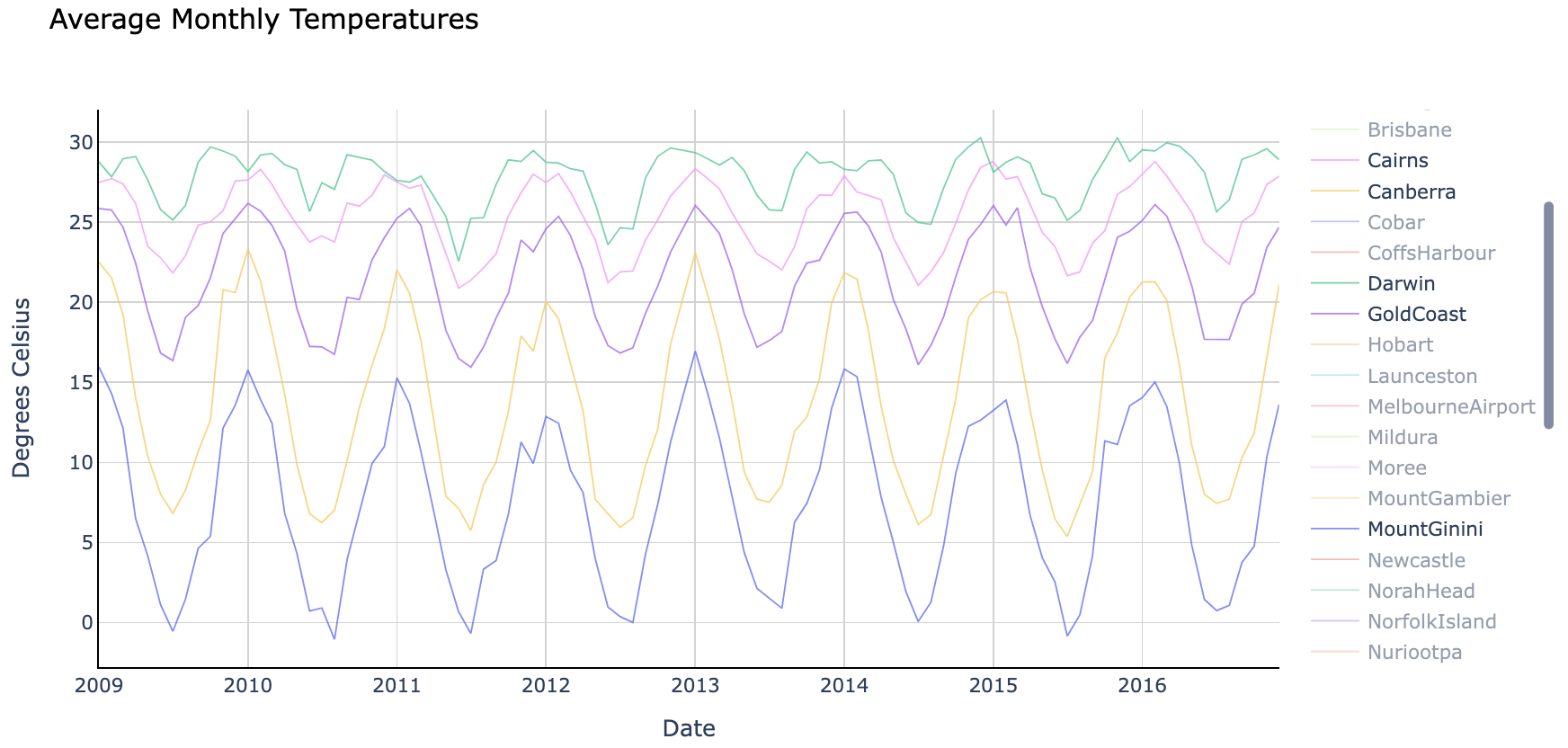 平均月温度。来源
图表最初显示所有地点,但我在上图中仅选取了五个(Cairns、Canberra、Darwin、Gold Coast 和 Mount Ginini)进行展示。
注意各地点的平均温度及其变化幅度各不相同。我们可以为每个地点训练特定模型以获得更高精度,也可以训练一个通用模型来预测所有地区的温度。
在本示例中,我将创建一个在所有地点上训练的通用模型。
训练和评估 GRU 模型
在开始之前,有几点需要强调:
- 我们将使用 18 个月的序列来预测接下来 18 个月的平均温度。你可以根据需要调整,但请注意,超过 23 个月的序列将没有足够数据。
- 我们将数据拆分为两个独立的数据框——一个用于训练,另一个用于验证(样本外验证)。
- 由于我们正在创建多对多预测模型,我们需要使用稍微复杂的编码器-解码器(encoder-decoder)配置。编码器和解码器都是隐藏的 GRU 层,通过 RepeatVector 层传递信息。
- 当输入和输出序列长度不同时(例如用 18 个月序列预测接下来 12 个月),RepeatVector 是必要的,它确保为解码器层提供正确的形状。但在本例中,输入和输出序列长度相同,因此你也可以选择在编码器层设置
return_sequences=True并移除 RepeatVector。 - 注意,我们在 GRU 层外添加了
Bidirectional包装器。它允许模型双向训练,有时效果更好,但使用它是可选的。 - 此外,我们需要在输出层使用
TimeDistributed包装器,以便为每个时间步单独预测输出。 - 最后,我在本例中使用了 MinMaxScaling,因为它比未缩放版本效果更好。你可以在我的 GitHub 仓库中的 Jupyter Notebook 中找到缩放和未缩放两种设置(文章末尾提供链接)。
首先,定义一个辅助函数,将数据重塑为 GRU 所需的 3D 数组。
def shaping(datain, timestep, scaler):

    # Loop through each location
    for location in datain.index:
        datatmp = datain[datain.index==location].copy()

        # Convert input dataframe to array and flatten
        arr=datatmp.to_numpy().flatten()

        # Scale using transform (using previously fitted scaler)
        arr_scaled=scaler.transform(arr.reshape(-1, 1)).flatten()

        cnt=0
        for mth in range(0, len(datatmp.columns)-(2*timestep)+1): # Define range
            cnt=cnt+1 # Gives us the number of samples. Later used to reshape the data
            X_start=mth # Start month for inputs of each sample
            X_end=mth+timestep # End month for inputs of each sample
            Y_start=mth+timestep # Start month for targets of each sample. Note, start is inclusive and end is exclusive, that's why X_end and Y_start is the same number
            Y_end=mth+2*timestep # End month for targets of each sample.

            # Assemble input and target arrays containing all samples
            if mth==0:
                X_comb=arr_scaled[X_start:X_end]
                Y_comb=arr_scaled[Y_start:Y_end]
            else:
                X_comb=np.append(X_comb, arr_scaled[X_start:X_end])
                Y_comb=np.append(Y_comb, arr_scaled[Y_start:Y_end])

        # Reshape input and target arrays
        X_loc=np.reshape(X_comb, (cnt, timestep, 1))
        Y_loc=np.reshape(Y_comb, (cnt, timestep, 1))

        # Append an array for each location to the master array
        if location==datain.index[0]:
            X_out=X_loc
            Y_out=Y_loc
        else:
            X_out=np.concatenate((X_out, X_loc), axis=0)
            Y_out=np.concatenate((Y_out, Y_loc), axis=0)

    return X_out, Y_out
接下来,我们在 50 个 epoch 上训练 GRU 神经网络,并显示模型摘要和评估指标。你可以通过代码中的注释理解每一步。
##### Step 1 - Specify parameters
timestep=18
scaler = MinMaxScaler(feature_range=(-1, 1))

##### Step 2 - Prepare data

# Split data into train and test dataframes
df_train=df2_pivot.iloc[:, 0:-2*timestep].copy()
df_test=df2_pivot.iloc[:, -2*timestep:].copy()

# Use fit to train the scaler on the training data only, actual scaling will be done inside reshaping function
scaler.fit(df_train.to_numpy().reshape(-1, 1))

# Use previously defined shaping function to reshape the data for GRU
X_train, Y_train = shaping(datain=df_train, timestep=timestep, scaler=scaler)
X_test, Y_test = shaping(datain=df_test, timestep=timestep, scaler=scaler)

##### Step 3 - Specify the structure of a Neural Network
model = Sequential(name="GRU-Model") # Model
model.add(Input(shape=(X_train.shape[1],X_train.shape[2]), name='Input-Layer')) # Input Layer - need to speicfy the shape of inputs
model.add(Bidirectional(GRU(units=32, activation='tanh', recurrent_activation='sigmoid', stateful=False), name='Hidden-GRU-Encoder-Layer')) # Encoder Layer
model.add(RepeatVector(X_train.shape[1], name='Repeat-Vector-Layer')) # Repeat Vector
model.add(Bidirectional(GRU(units=32, activation='tanh', recurrent_activation='sigmoid', stateful=False, return_sequences=True), name='Hidden-GRU-Decoder-Layer')) # Decoder Layer
model.add(TimeDistributed(Dense(units=1, activation='linear'), name='Output-Layer')) # Output Layer, Linear(x) = x

##### Step 4 - Compile the model
model.compile(optimizer='adam', # default='rmsprop', an algorithm to be used in backpropagation
              loss='mean_squared_error', # Loss function to be optimized. A string (name of loss function), or a tf.keras.losses.Loss instance.
              metrics=['MeanSquaredError', 'MeanAbsoluteError'], # List of metrics to be evaluated by the model during training and testing. Each of this can be a string (name of a built-in function), function or a tf.keras.metrics.Metric instance.
              loss_weights=None, # default=None, Optional list or dictionary specifying scalar coefficients (Python floats) to weight the loss contributions of different model outputs.
              weighted_metrics=None, # default=None, List of metrics to be evaluated and weighted by sample_weight or class_weight during training and testing.
              run_eagerly=None, # Defaults to False. If True, this Model's logic will not be wrapped in a tf.function. Recommended to leave this as None unless your Model cannot be run inside a tf.function.
              steps_per_execution=None # Defaults to 1. The number of batches to run during each tf.function call. Running multiple batches inside a single tf.function call can greatly improve performance on TPUs or small models with a large Python overhead.
             )

##### Step 5 - Fit the model on the dataset
history = model.fit(X_train, # input data
                    Y_train, # target data
                    batch_size=1, # Number of samples per gradient update. If unspecified, batch_size will default to 32.
                    epochs=50, # default=1, Number of epochs to train the model. An epoch is an iteration over the entire x and y data provided
                    verbose=1, # default='auto', ('auto', 0, 1, or 2). Verbosity mode. 0 = silent, 1 = progress bar, 2 = one line per epoch. 'auto' defaults to 1 for most cases, but 2 when used with ParameterServerStrategy.
                    callbacks=None, # default=None, list of callbacks to apply during training. See tf.keras.callbacks
                    validation_split=0.2, # default=0.0, Fraction of the training data to be used as validation data. The model will set apart this fraction of the training data, will not train on it, and will evaluate the loss and any model metrics on this data at the end of each epoch.
                    #validation_data=(X_test, y_test), # default=None, Data on which to evaluate the loss and any model metrics at the end of each epoch.
                    shuffle=True, # default=True, Boolean (whether to shuffle the training data before each epoch) or str (for 'batch').
                    class_weight=None, # default=None, Optional dictionary mapping class indices (integers) to a weight (float) value, used for weighting the loss function (during training only). This can be useful to tell the model to "pay more attention" to samples from an under-represented class.
                    sample_weight=None, # default=None, Optional Numpy array of weights for the training samples, used for weighting the loss function (during training only).
                    initial_epoch=0, # Integer, default=0, Epoch at which to start training (useful for resuming a previous training run).
                    steps_per_epoch=None, # Integer or None, default=None, Total number of steps (batches of samples) before declaring one epoch finished and starting the next epoch. When training with input tensors such as TensorFlow data tensors, the default None is equal to the number of samples in your dataset divided by the batch size, or 1 if that cannot be determined.
                    validation_steps=None, # Only relevant if validation_data is provided and is a tf.data dataset. Total number of steps (batches of samples) to draw before stopping when performing validation at the end of every epoch.
                    validation_batch_size=None, # Integer or None, default=None, Number of samples per validation batch. If unspecified, will default to batch_size.
                    validation_freq=10, # default=1, Only relevant if validation data is provided. If an integer, specifies how many training epochs to run before a new validation run is performed, e.g. validation_freq=2 runs validation every 2 epochs.
                    max_queue_size=10, # default=10, Used for generator or keras.utils.Sequence input only. Maximum size for the generator queue. If unspecified, max_queue_size will default to 10.
                    workers=1, # default=1, Used for generator or keras.utils.Sequence input only. Maximum number of processes to spin up when using process-based threading. If unspecified, workers will default to 1.
                    use_multiprocessing=True, # default=False, Used for generator or keras.utils.Sequence input only. If True, use process-based threading. If unspecified, use_multiprocessing will default to False.
                   )

##### Step 6 - Use model to make predictions
# Predict results on training data
#pred_train = model.predict(X_train)
# Predict results on test data
pred_test = model.predict(X_test)

##### Step 7 - Print Performance Summary
print("")
print('-------------------- Model Summary --------------------')
model.summary() # print model summary
print("")
print('-------------------- Weights and Biases --------------------')
print("Too many parameters to print but you can use the code provided if needed")
print("")
#for layer in model.layers:
#    print(layer.name)
#    for item in layer.get_weights():
#        print("  ", item)
#print("")

# Print the last value in the evaluation metrics contained within history file
print('-------------------- Evaluation on Training Data --------------------')
for item in history.history:
    print("Final", item, ":", history.history[item][-1])
print("")

# Evaluate the model on the test data using "evaluate"
print('-------------------- Evaluation on Test Data --------------------')
results = model.evaluate(X_test, Y_test)
print("")
上述代码为我们的 GRU 神经网络打印了以下摘要和评估指标(注意,由于神经网络训练的随机性,你的结果可能有所不同):
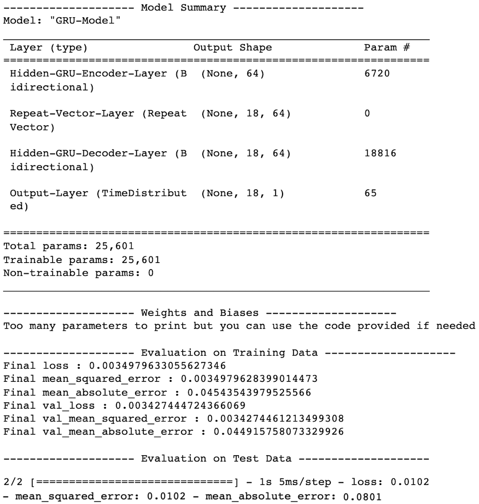 GRU 神经网络性能。来源
现在,让我们为我们之前选取的 5 个地点重新生成预测,并将结果绘制在图表上,以比较实际值和预测值。
预测
# Select locations to predict temperatures for
location=['Cairns', 'Canberra', 'Darwin', 'GoldCoast', 'MountGinini']
dfloc_test = df_test[df_test.index.isin(location)].copy()

# Reshape test data
X_test, Y_test = shaping(datain=dfloc_test, timestep=timestep, scaler=scaler)

# Predict results on test data
pred_test = model.predict(X_test)
绘图
# Plot average monthly temperatures (actual and predicted) for test (out of time) data
fig = go.Figure()

# Trace for actual temperatures
for location in dfloc_test.index:
    fig.add_trace(go.Scatter(x=dfloc_test.loc[location, :].index,
                             y=dfloc_test.loc[location, :].values,
                             mode='lines',
                             name=location,
                             opacity=0.8,
                             line=dict(width=1)
                            ))

# Trace for predicted temperatures
for i in range(0,pred_test.shape[0]):
    fig.add_trace(go.Scatter(x=np.array(dfloc_test.columns[-timestep:]),
                             # Need to inverse transform the predictions before plotting
                             y=scaler.inverse_transform(pred_test[i].reshape(-1,1)).flatten(),
                             mode='lines',
                             name=dfloc_test.index[i]+' Prediction',
                             opacity=1,
                             line=dict(width=2, dash='dot')
                            ))

# Change chart background color
fig.update_layout(dict(plot_bgcolor = 'white'))

# Update axes lines
fig.update_xaxes(showgrid=True, gridwidth=1, gridcolor='lightgrey',
                 zeroline=True, zerolinewidth=1, zerolinecolor='lightgrey',
                 showline=True, linewidth=1, linecolor='black',
                 title='Year-Month'
                )

fig.update_yaxes(showgrid=True, gridwidth=1, gridcolor='lightgrey',
                 zeroline=True, zerolinewidth=1, zerolinecolor='lightgrey',
                 showline=True, linewidth=1, linecolor='black',
                 title='Degrees Celsius'
                )

# Set figure title
fig.update_layout(title=dict(text="Average Monthly Temperatures", font=dict(color='black')))
fig.show()
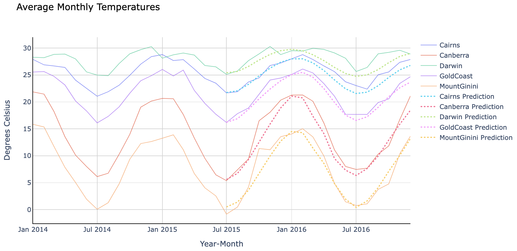 GRU 神经网络预测 vs. 实际值。来源
看起来我们的 GRU 模型很好地捕捉了每个地点的温度趋势!
最后说明
GRU 和 LSTM 不仅在架构上相似,在预测能力上也相近。因此,在选择你最喜欢的模型之前,不妨两者都试试。
如果你想获取完整的 Python 代码,可以在我的 GitHub 仓库中找到 Jupyter Notebook。
感谢阅读!如果你有任何问题或建议,欢迎随时联系我。
干杯!